I have time series data of 60 different emotional states that I’ve recorded daily for about 6 years. I’ve explored a few methods for classifying these states, most recently with PCA, or principal component analysis. My goal is to simplify the 60 states into a smaller number of components or dimensions that describe my emotional state. In this case, 25 components described 80% of the variance in the data. There was no labeling of the data, or subjective rule-making, only the PCA determining the most important vectors that describe the data; starting with the first two components, PC1 and PC2.
Read MoreCo-Authorship with AI
Some thoughts on the question of authorship when using generative AI tools.
TLDR: I think it’s most prudent to provide a short list of collaborators, rather than a sole author. For example, list the relevant Primary Author / Product / Model / Training Data.

ie: Adam Heisserer/ StyleGAN2 / GAN
Who wrote the song ‘Yesterday’? One morning, Paul McCartney woke up with the tune in his head. It sounded so familiar, he assumed he was remembering a pre-existing tune. After a while, he accepted that it was not a pre-existing song, but a novel one that appeared to him. So who wrote it? Was it Paul McCartney, who spent a lifetime crafting and listening to music? This is the equivalent of training data and the latent space that makes up all the potential songs that could be, based on what he knows about the structure and characteristics of all songs. Was it Paul’s sleeping subconscious brain that wrote it? In part, yes. Or was it waking Paul, who had the wherewithal to recognize, remember and record the tune after consciously authoring the lyrics? I’d say it was all three. Because there’s not much of a legal distinction between Paul and his subconscious sleeping brain, it’s practical to just to name him the sole author.
When using generative AI tools to create images, there is a distinction between the human curator and the model ‘dreamer’. More of a co-authorship that’s worth acknowledging. Further distinction could be made to include who authored, and who curated the training data. Or, who crafted the exact generative process.
If there’s a question of authorship, list multiple co-authors. Don’t be dishonest, but don’t overthink it. Because of their generative nature and vast training data, this includes generative AI image models.
Graphing Multiple Moving Averages with Python
Multiple moving averages
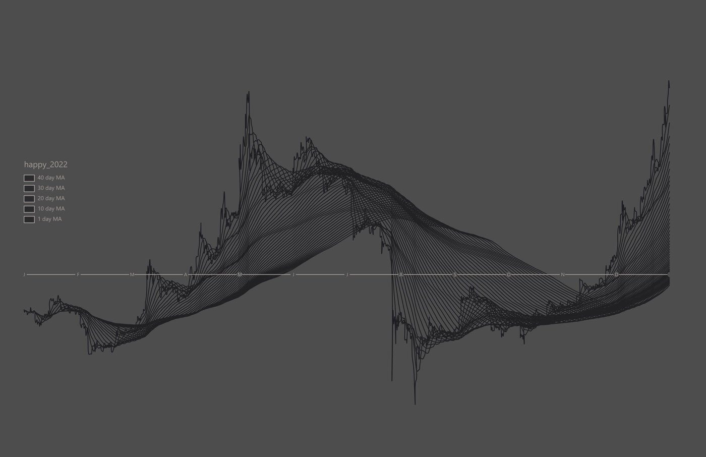
Multiple moving average graph
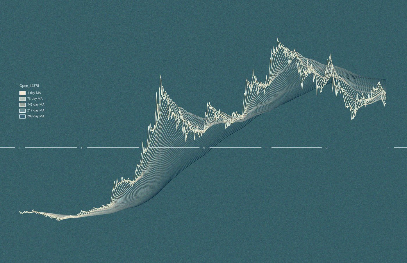
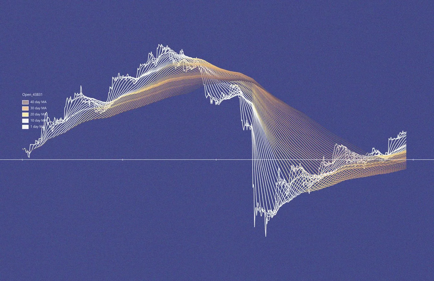


Image to Image Translation with Stable Diffusion
These are experiments in using Stable Diffusion as an image-to-image pipeline. Essentially, a kind of image style transfer using text prompts.
I’m using this huggingface/diffusers repository: https://github.com/huggingface/diffusers
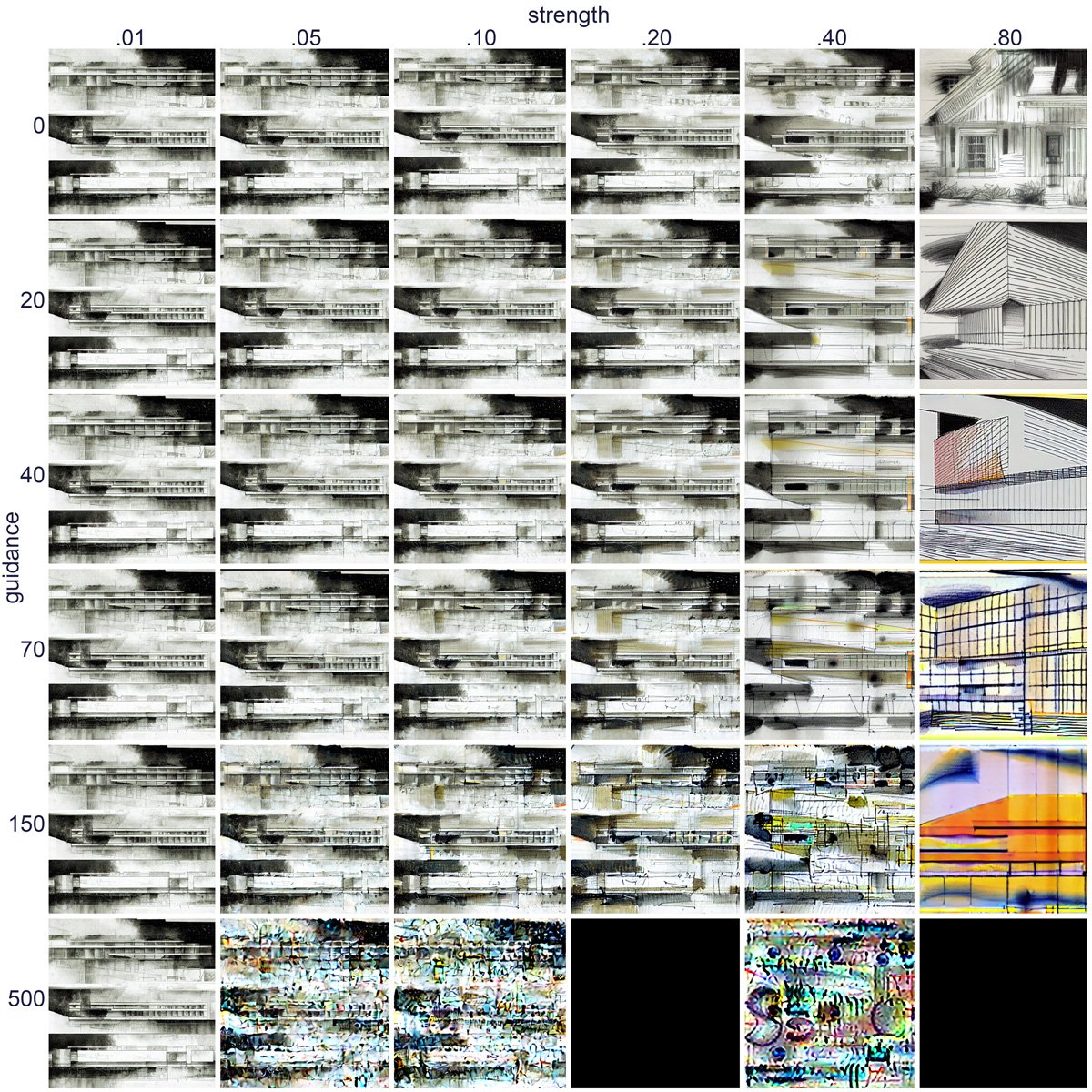
The stable diffusion model takes an initial image, a text prompt, a random seed, a strength value, and a guidance scale value. The following grid shows the results of passing an image through varying strength and guidance scales, all with the same text prompt and seed. The randomly generated prompt in this case is: “a page of yellow section perspective with faint orange lines”.
An increasing strength value adds greater variation to the initial image. At less than 0.05, it hardly effects the initial image, but past .50, it starts to become unrecognizable.
An increasing guidance scale increases the adherence of the image to the prompt. Beyond 100, the image quality becomes… radical.
Some squares get blacked out because some aspect of the generated image gets flagged as potentially NSFW. This is more common with high strength and guidance values.
I readjusted the range of both strength and guidance, regenerated the prompt to: "detailed architectural photograph with minimalist circular people everywhere", and tried a new initial image.

The following are made with a random seed and randomly generated prompt for each iteration. The prompts are built with variable adjectives, subjects, drawing types, drawing mediums, etc, generally architectural in nature.


This range tends to be the best for the kind of image style transfer I’m looking for. Anything to the left is too similar to the original image, and anything to the right is too different.

StyleGAN2 + CLIP Guided Diffusion
StyleGAN and CLIP + Guided Diffusion are two different tools for generating images, each with their own relative strengths and weaknesses. This is an experiment in pairing the two to get a result that’s better than using one or the other.
What does StyleGAN do? It takes a set of images and produces novel images that belong to the same class. It’s most successful when the image set is relatively uniform, such as faces, flowers, landscapes, etc, where the same features reoccur in every instance of the class. When the image set becomes to diverse, such as this set of architectural drawings, the results are more abstract. Even with abstract results, the compositions are still striking.
What does CLIP + Guided Diffusion do? CLIP (Contrastive Language-Image Pretraining) is a text-guide, where the user inputs a prompt, and the image is influenced by the text description. Diffusion models can be thought of as an additive process where random noise is added to an image, and the model interprets the noise into a rational image. These models tend to produce a wider range of results than adversarial GAN models.
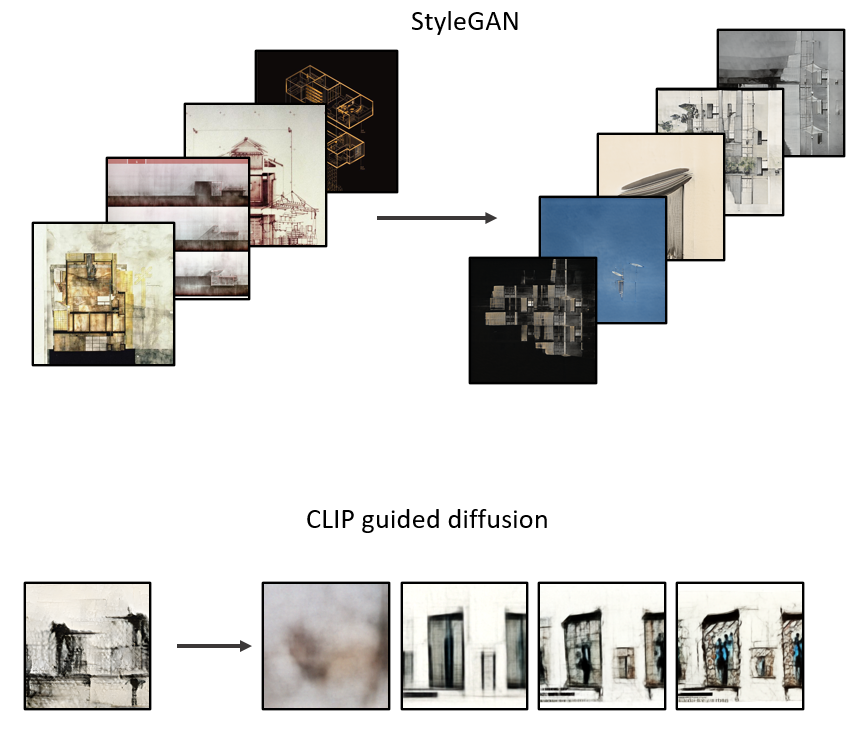
The goal is to keep the striking and abstract compositions from StyleGAN, and then feed those results into a Guided Diffusion model for a short time, so the original image gains some substance or character while ‘painting over’ some of the artifacts that give away the image as a coming from StyleGAN.
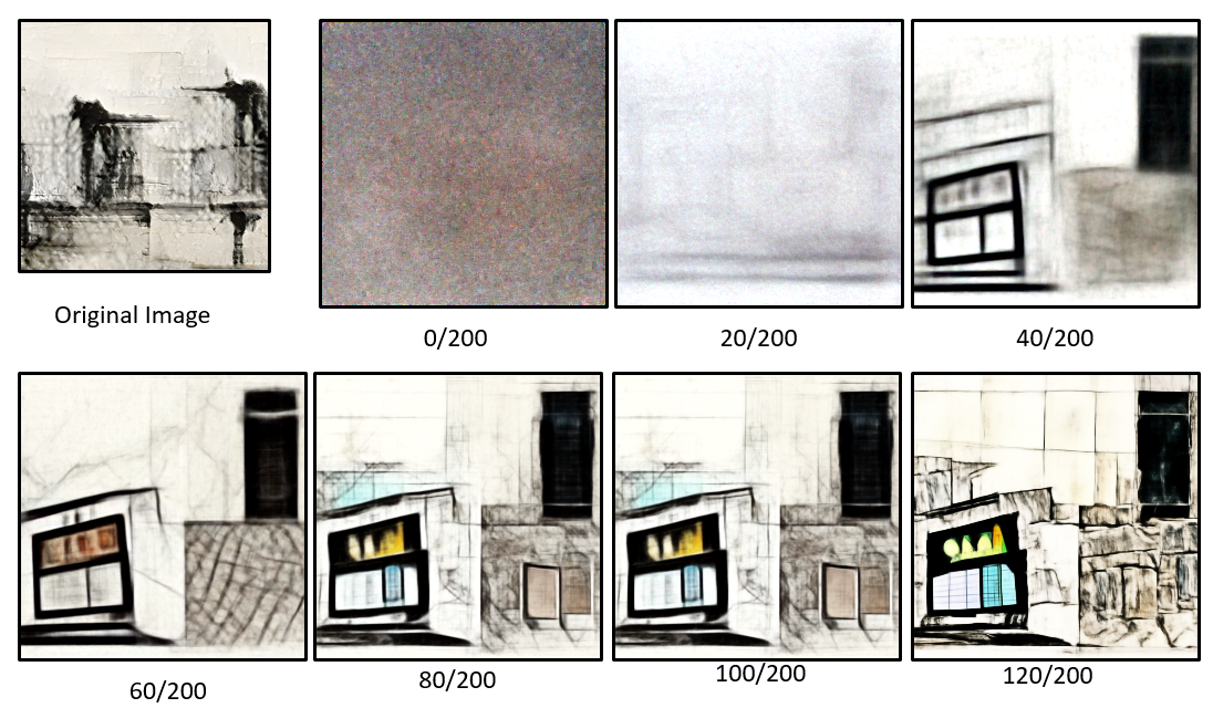
This is a typical Guided Diffusion process from beginning to end. Gaussian noise is added to an image, and then the image is de-noised, imagining new objects. This de-noising process continues, adding definition and detail to the objects imagined by the model.
The diffusion model can start with an input image, skipping some of the early steps of the model. This way, the final image retains the broad strokes of the original input image.
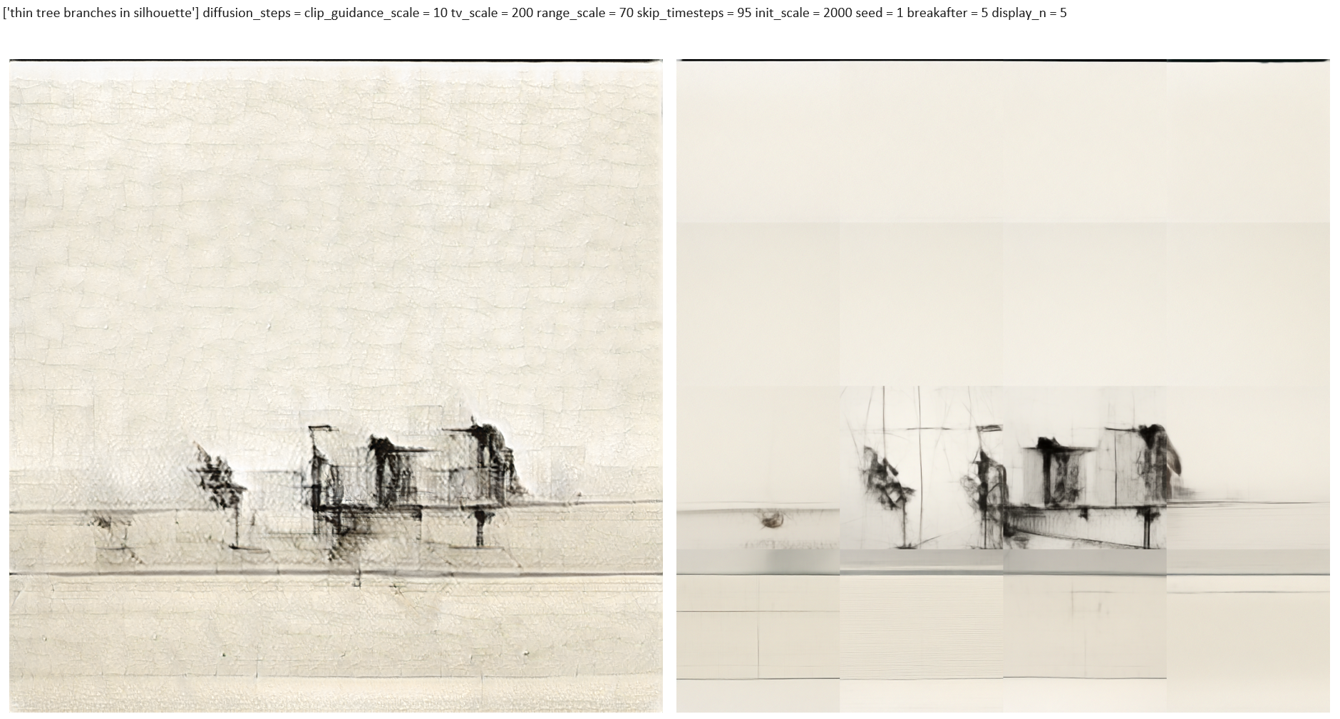
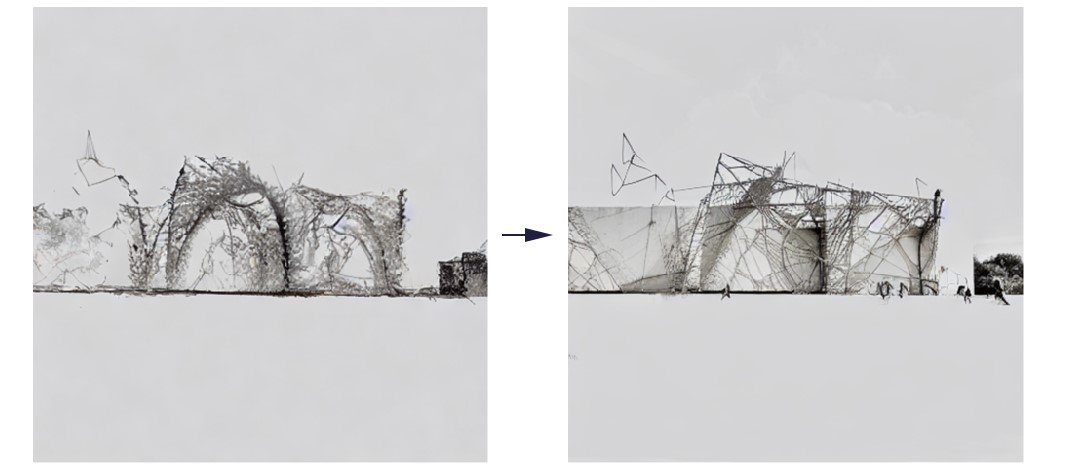
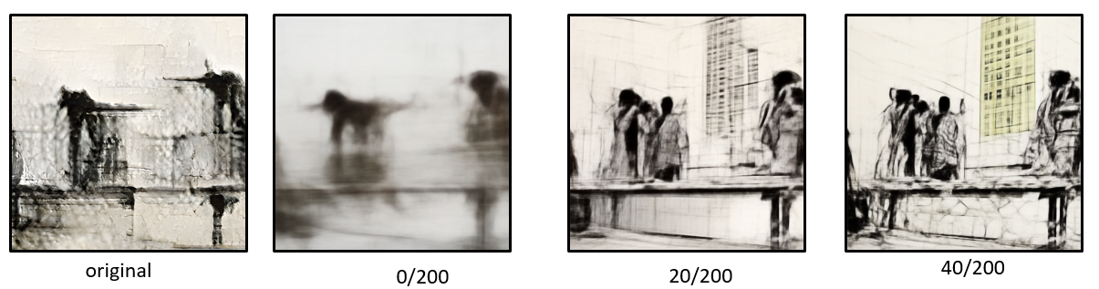
The image on the left is the output from a StyleGAN model, trained on an image set of architectural drawings. This original image was split into 16 segments, each of which were processed with CLIP + Guided Diffusion. The overall composition remains intact, while the diffusion model re-renders each block of the original image, taking away the texture and artifacts from the original. The result is a higher resolution image than the original. The downside is the inconsistency of splitting the image into 16 sections.
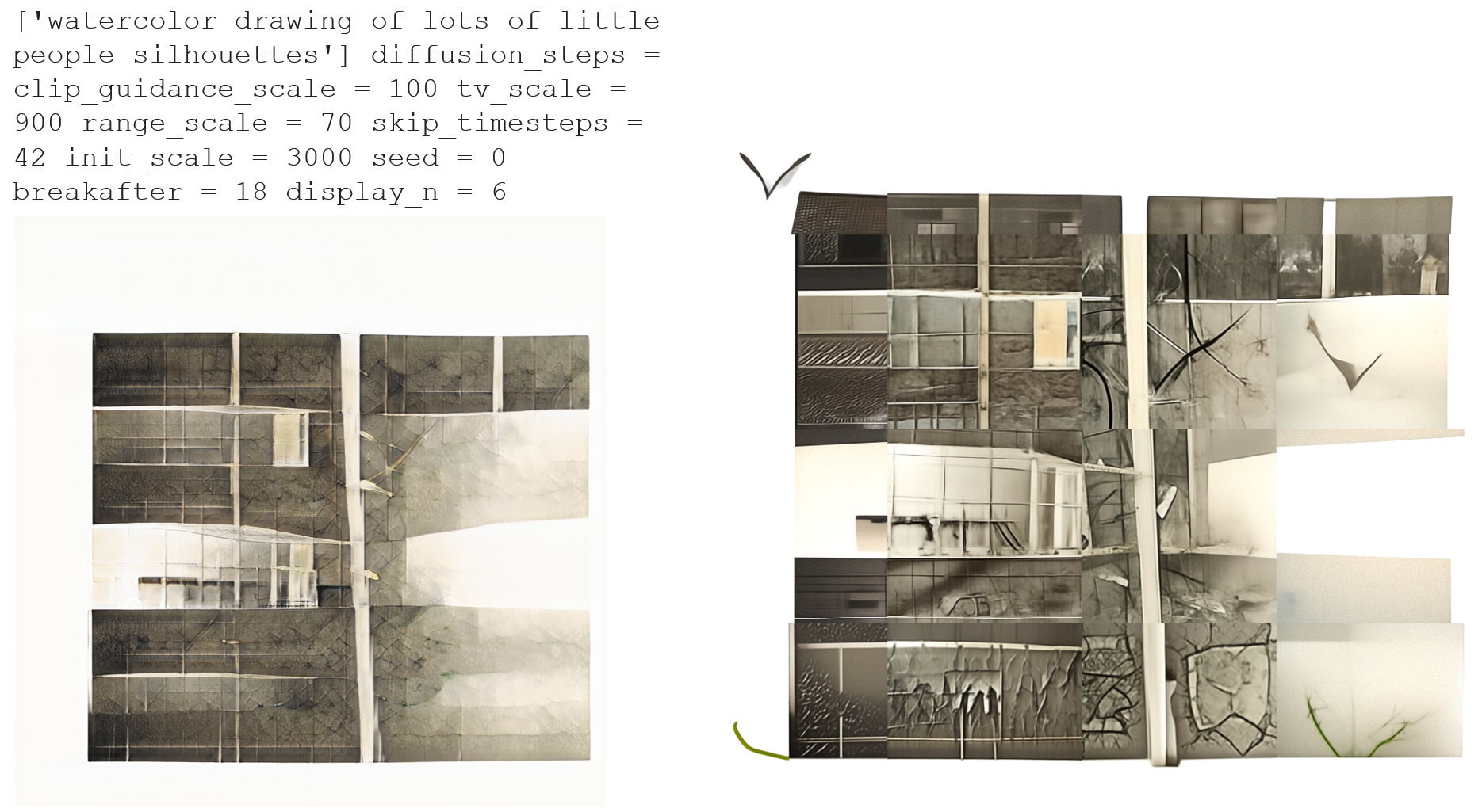
This is another example of splitting an original StyleGAN image into 16 squares, and re-rendering in CLIP + Guided Diffusion. I was hoping the guided diffusion model would add more definition and substance to the original. I suppose it did, but it lacks consistency and realism.
Music Blocks
This is an ongoing project about taking a large data set of songs, converting them all to the same key and tempo, and then mixing and matching clips of different songs to generate new sounds and ideas for songwriting. This is the process so far:
1: Collect a data set of music.
I collected about 1,000 song and made a separate copy, leaving all the original files untouched. I converted all of the files to .MP3 format, and filtered out any files over 20MB. I used freeware called mp3tag to extract all the metadata from the data set, and made an Excel spreadsheet with all song metadata.
2. Identify the Key and Tempo of each song.
I used a python library called Madmom to identify the key of each song (major or minor, and the root of the chord). This wasn’t perfectly accurate for all songs, but it was close. Next, I use Madmom to extract the beats and downbeats in each song, and estimate the tempo. A lot of songs have variable tempos, so I wrote something to find the max and min tempo and filtered out all the songs that varied too much in tempo. Now key and tempo are added to the Excel data set.
3. Convert all songs to be the same tempo and Pitch
I used the ffmpeg library to convert all songs to the identical pitch and tempo (100bpm). This strongly distorts some of the tracks. Optionally, I can filter out the songs that were too distorted.
4. Split each song into 4-bar clips, each 10 seconds long.
Using the downbeat detection from earlier, I used ffmpeg to split each of the pitch/tempo-adjusted tracks into 4-bar clips. Each is 16 beats total, and exactly 10 seconds, because all songs are 100 beats per minute.
5. Mix and match
Now I have thousands of 10-second clips from hundreds of songs, each of which are theoretically in the same key and the same tempo. Practically, there are many inaccuracies in the previous steps, so quite a lot of the final clips are not accurately transformed. That’s why we start with so many songs, because they will inevitably get whittled down to a few that actually work.
At this point, I select several clips at random and drop them into Audacity, a simple audio mixing platform. I play several clips simultaneously on a loop, and mix the volume, highlighting interesting combinations and moments, and excluding clips that don’t work with the mix. Sometimes I get interesting combinations of clips, such as this mix of two Borns clips, from “Fool”, “Past Lives” and a few other songs in the background.
It’s kind of muddy and chaotic, but the idea is to discover interesting moments, like the last couple of seconds of the clip, where the arrangement gets thin and the few parts work well together.
What’s Next
I’ve also used a library called Demucs that isolates vocals, drums, bass, and all other instrumentation. I could further split these clips into separate tracks. The ultimate goal of all of this is to build a large database of 10-second clips, or “blocks” of 4 bars of music, separated by source (vocals, drums, bass, etc). These can be converted into a spectrogram, or a visual representation of frequencies over time. These could then be used to train a GAN to produce novel spectrograms of typical 4-bar phrases of vocals, bass, etc, to learn their properties. Then the trick is converting that spectrogram back to audio, and we’re getting at artificially “composed” music. For now it’s a fun trick for mixing music to discover new ideas.

Analyzing Architectural Drawings with Hough Transform
The Hough Transform is a method for extracting features from an image, such as lines, circles, or ellipses. For example, the computer vision task of edge detection can identify edges, but doesn’t describe the properties of those edges, such as whether or not the edges form a line or if those lines converge on a vanishing point. The Hough Transform is typically used for tasks like lane detection in autonomous driving, but the same process can be applied to architectural drawings or photography to shed some light on the properties of the lines in those images.
These transformations are really fun to generate, and I’m hoping they can be useful for classifying drawings by their perspective. For example, I would like to be able to classify a dataset of architectural drawings into plans, perspectives, isometrics, etc., and this type of analysis may be necessary for getting a machine learning process to “understand” the nature of the linework in a drawing. This is also a prerequisite for using ML to synthesize realistic architectural drawings, which is my eventual goal.
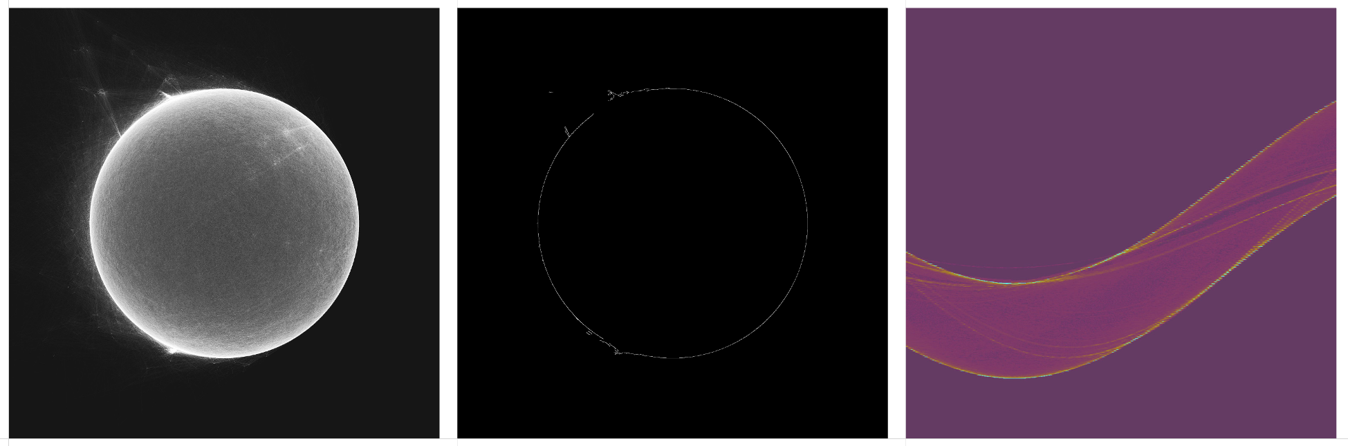
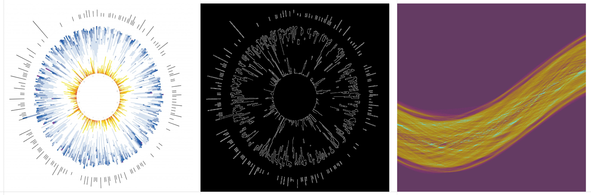
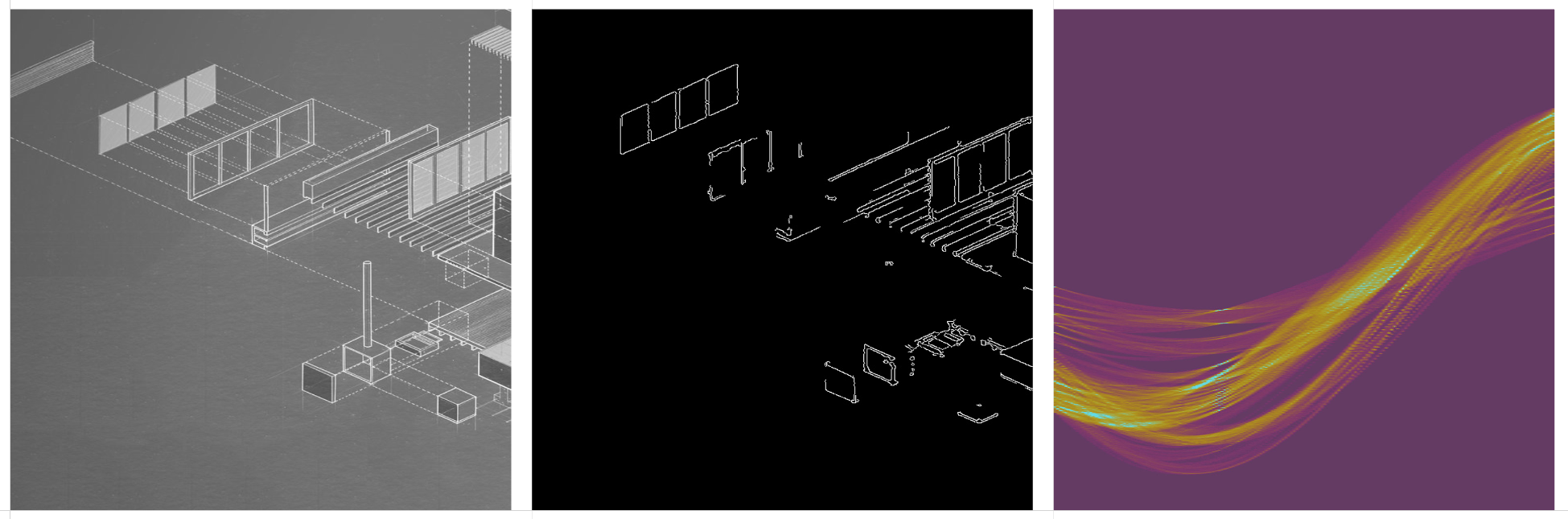
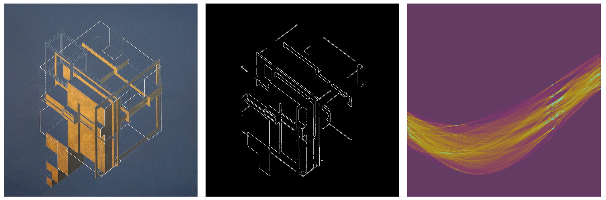
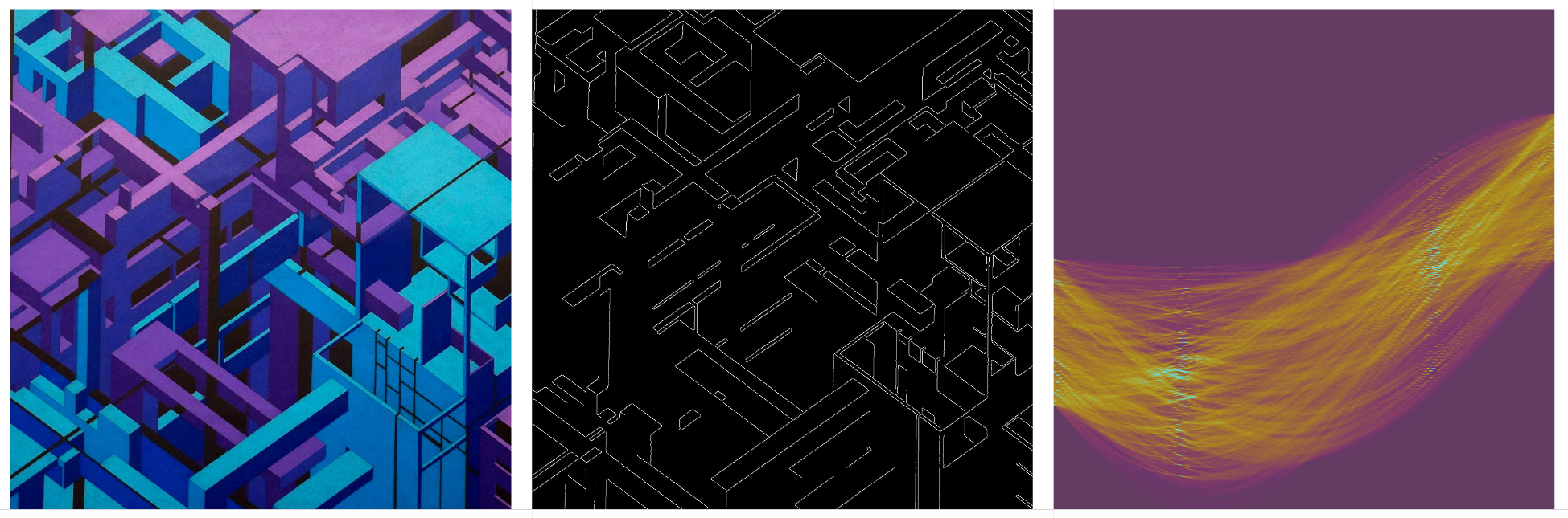
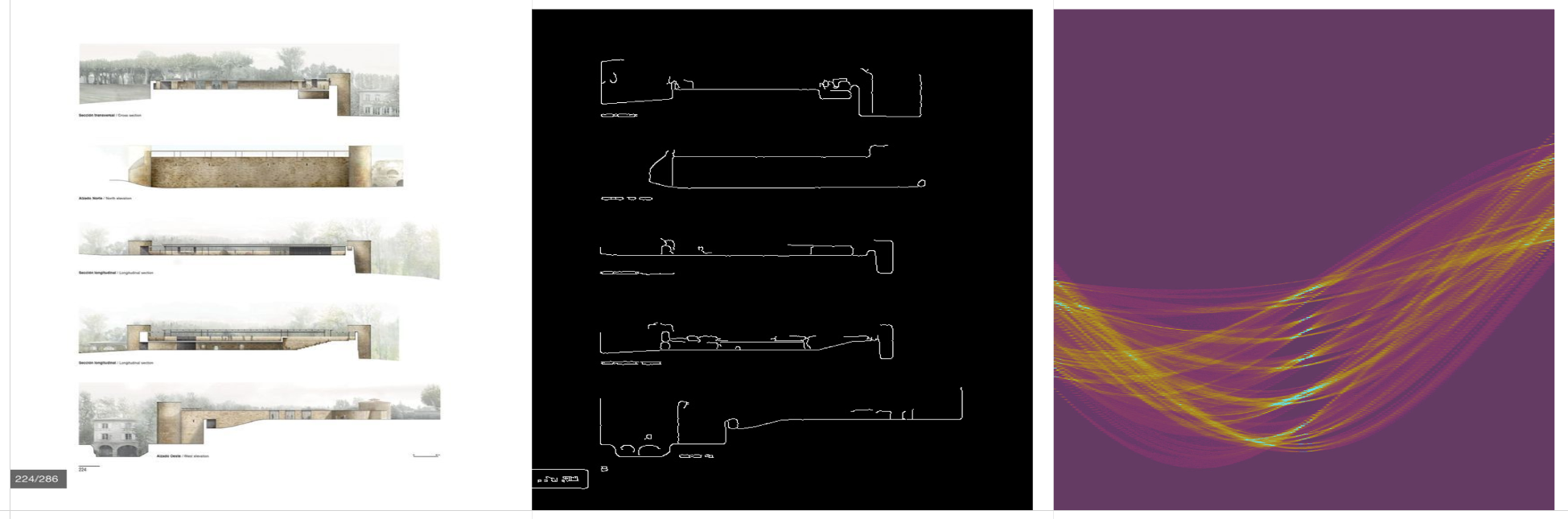
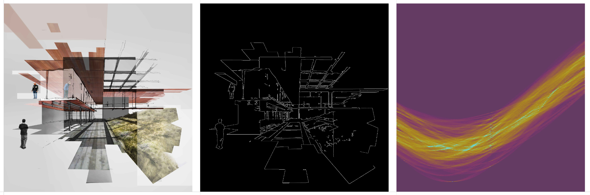
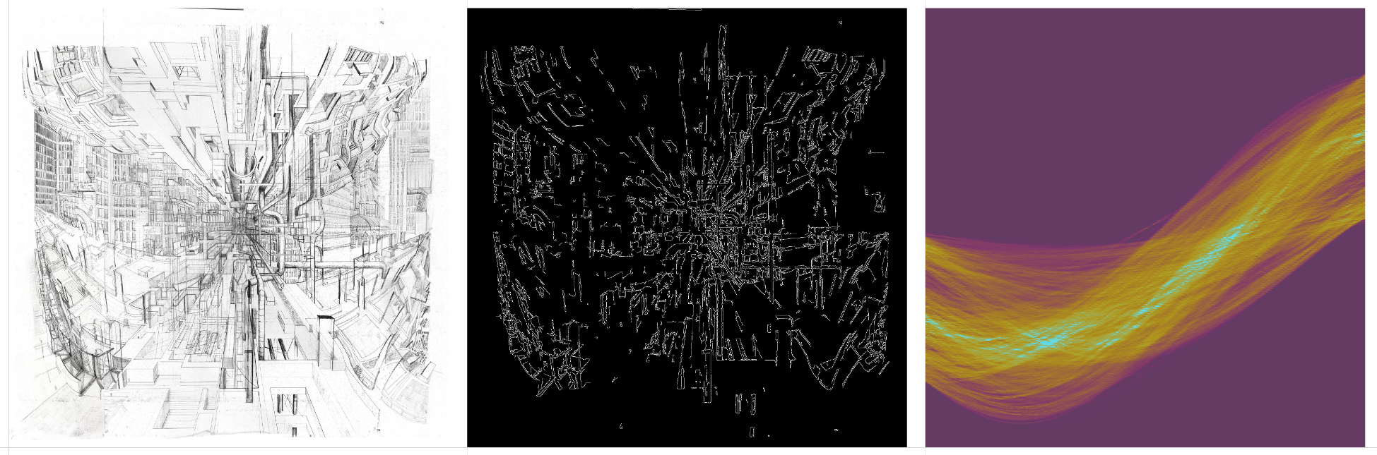
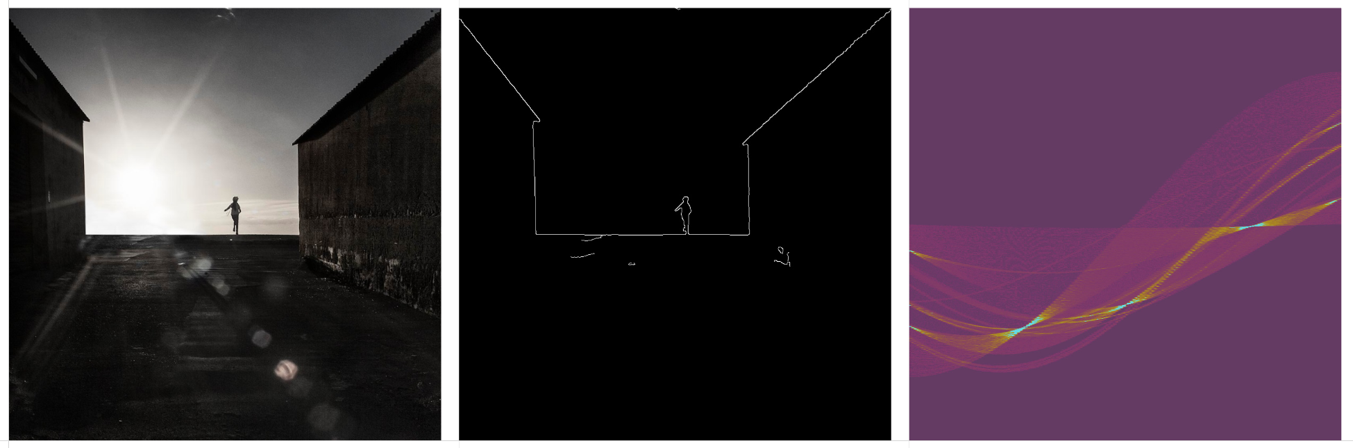
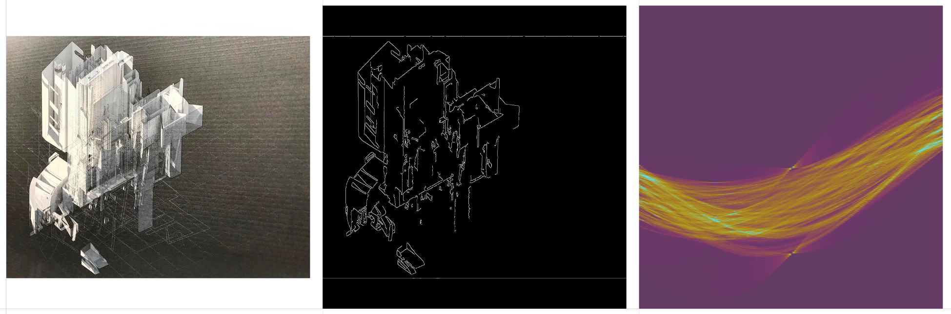
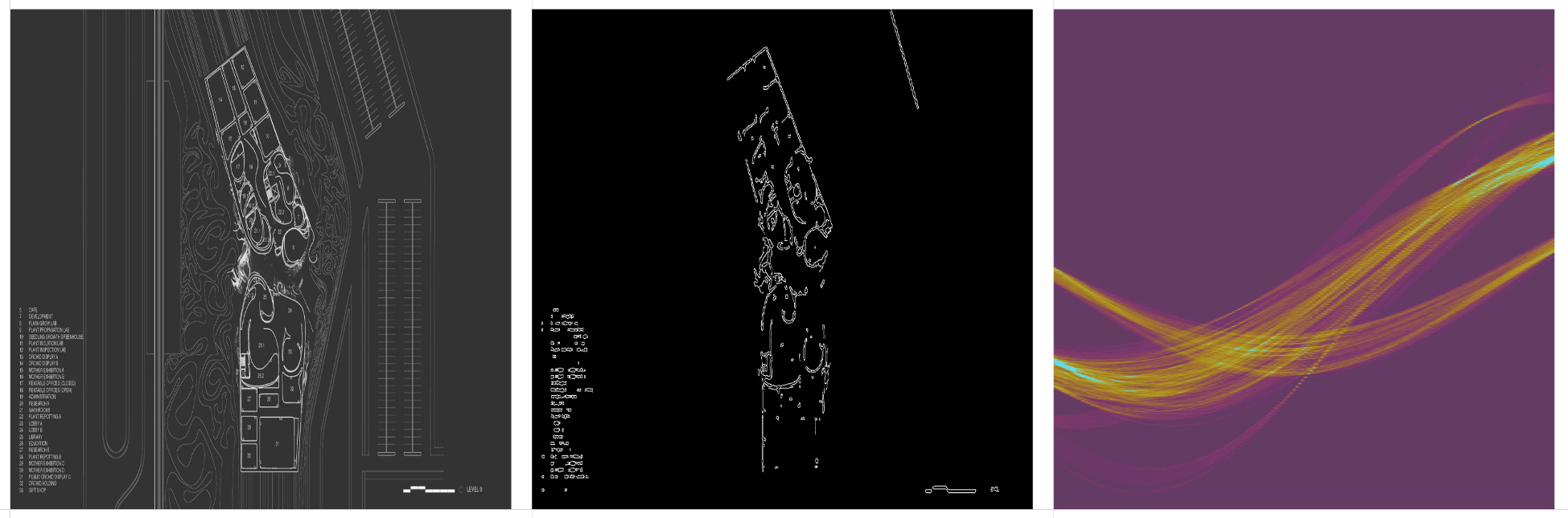
An oversimplification of how the transformation works: A drawing or photograph is processed with Canny edge detection. This extracts the high-contrast edges in an image. These edges are rendered as individual points, or pixels, not as true vectors or lines. Each point of the edge is converted from (x, y) coordinates to a series of (r, θ) coordinates, where r describes the distance from the center of the image to the nearest point on a line, and θ describes the angle of that line. The result is that every point on the edge is represented as a sinusoidal curve on a Hough Transform matrix. When these sine curves converge at a single point, it indicates that they describe a straight line.
This demo helps for building an intuition for the process. To put it simply, it’s a matter of representing points as lines, and lines as points.

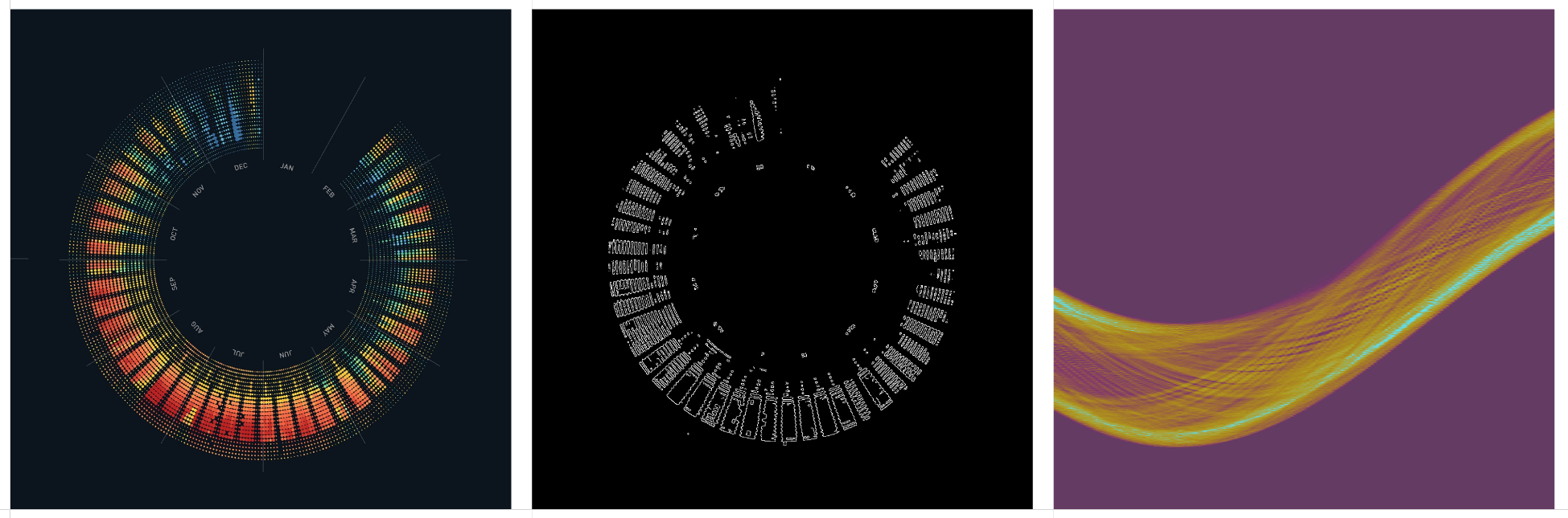
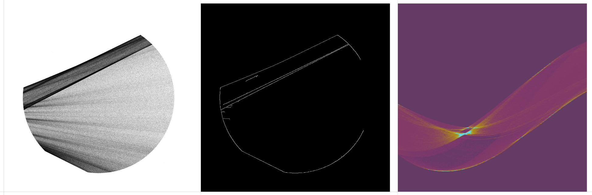
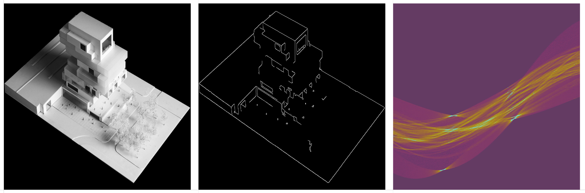
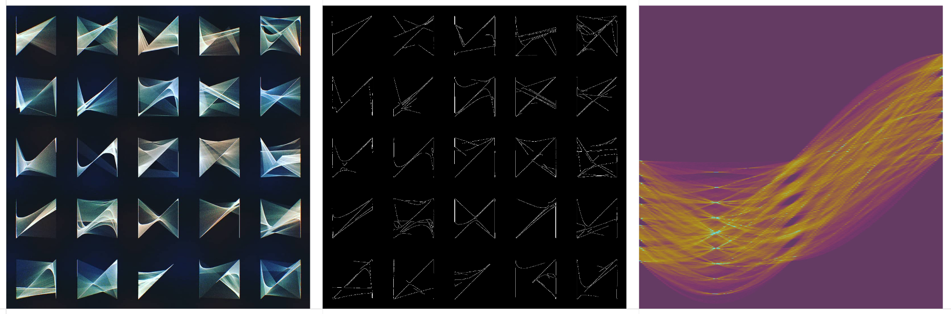
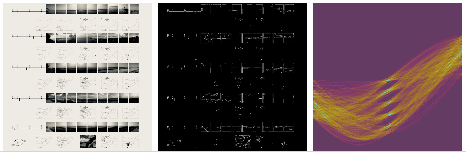
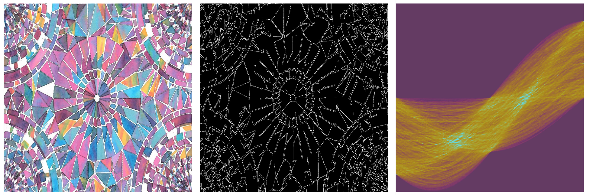
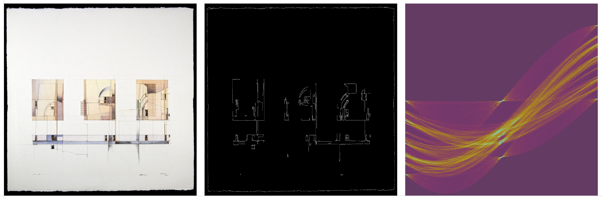
Original drawing, Canny edge detection, and the Hough Transform matrix.
Radial drawings produce a distinct band of curves. A perfect circle produces a perfect sine curve band, with hard edges. The middle point of the circle is indicated by the curve along the middle of the band.
Isometric drawings produce one or two vertical bands on the HT matrix, where the sine curves converge. The “x-axis” on the HT matrix is now the “theta” axis after the transformation, indicating the slope of each line, so isometric drawings will produce a vertical band on the left and right of center because of all of the parallel lines at about 45 degrees and -45 degrees. Notice the vertical bands on the last drawing are not perfectly vertical because the drawing is not a true isometric, but a 2 point perspective.
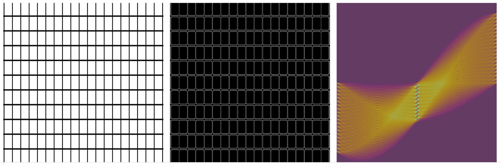
These gridded, orthogonal drawings have a distinct vertical band at the center of the “x-axis”. This falls at the theta=0 point, meaning the lines are horizontal. In the first drawing, which has no horizontal lines, the central vertical band isn’t showing converging points, but a lack of lines at intervals.
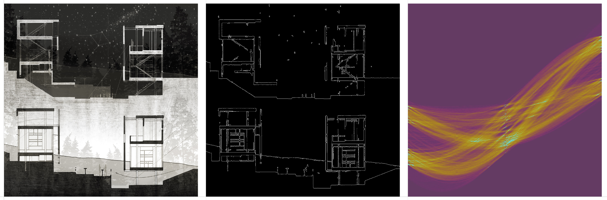
One point perspective drawings are difficult to characterize by their HT matrix. Lines that converge upon a single vanishing point appear as an implied sine curve in HT space. I say implied, because there’s a lot of linework that adds noise to the curve, and often the perspective lines don’t actually extend all the way to the vanishing point.
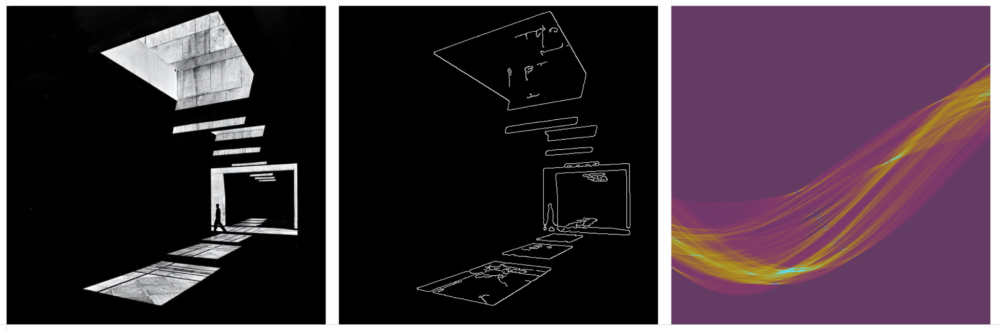
Borders are common on architectural drawings, and they show up as little flares in the HT space. See the convergences on the center line, above and below most of the linework. These indicate horizontal page borders at the top or bottom of the drawing.

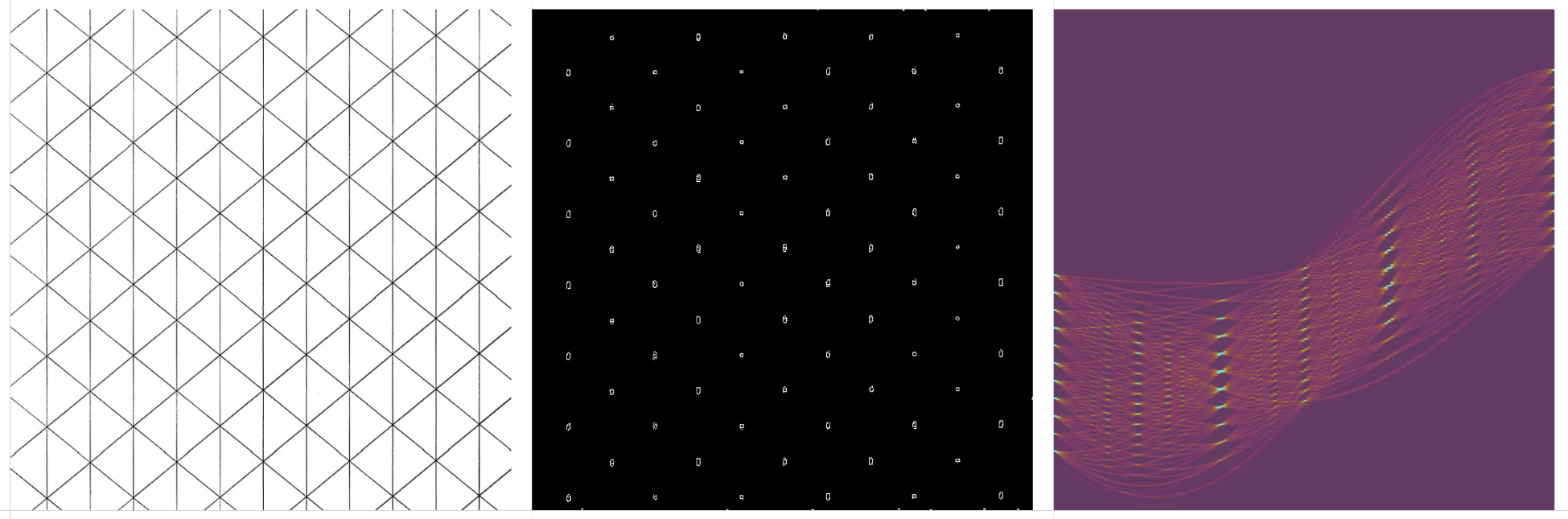
Here are some pure grids and their HT counterparts. The orthogonal grid has a vertical band of converging lines at the center (horizontal lines), and converging lines at the edge of the matrix (vertical lines). The isometric grid, in which Canny edge detection only picked up the nodes, has a few different vertical bands, indicating the multiple angles at which the nodes on the grid align.
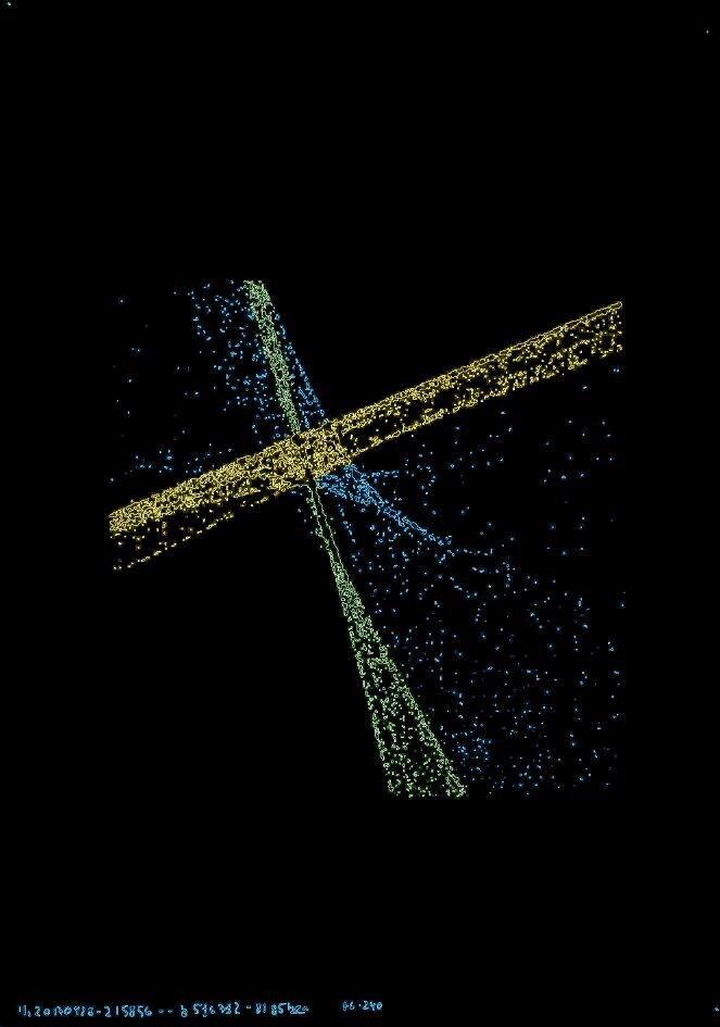
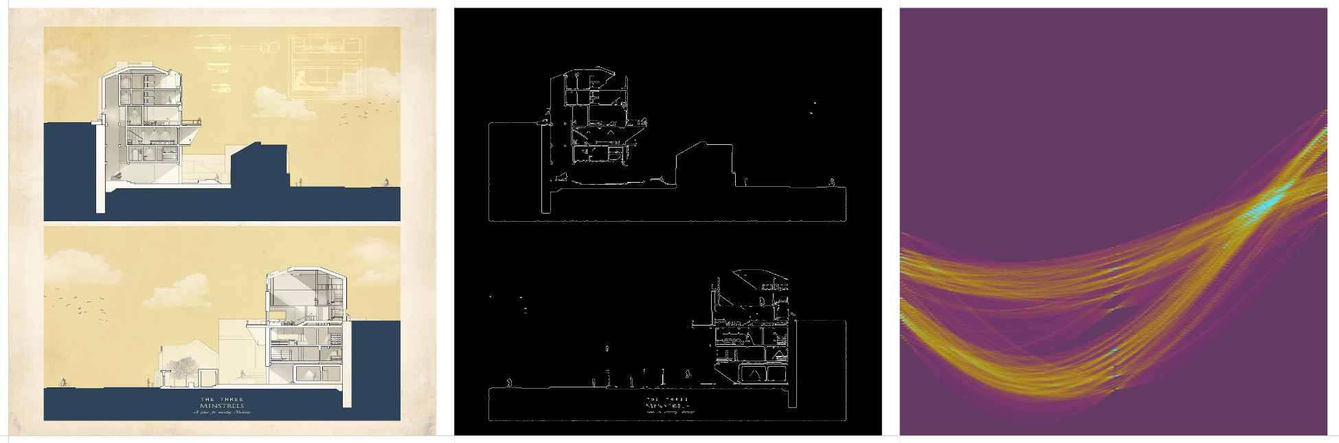
This is a color-coded drawing, with the HT bands colored respectively. The yellow band has a bright convergence slightly left of center (from a slightly positive slope of yellow lines in the drawing), and the green band has a convergence on the right which describes its slope. Notice the blue line, converging at the center (theta=0) point of the matrix, which came from the horizontal line of text at the bottom of the drawing.
Here are some interesting honorable mentions.
The Hough Transform was done with this Google Colab Notebook by Yoni Chechik, with a few modifications.
I use Derrick Schultz’s dataset tools to do Canny edge detection.
The coloring of the HT matrices were done with a gradient filter in Photoshop.
Using a Rhino Environment to Train a Surface-Normal Prediction Model in Pix2PixHD
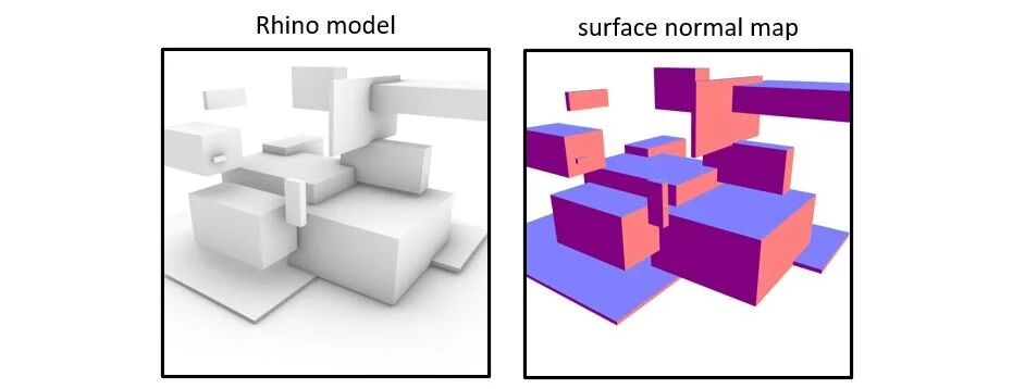
My goal is to train a Pix2PixHD model that can take an architectural drawing and synthesize a surface normal map. Surface normal mapping can be done in a Rhino/Grasshopper environment by taking a model, deconstructing it into a mesh, and coloring the surfaces so that each orientation is displayed with a different color. This is the type of analysis that I want to apply to any raw image.
Creating the Rhino Dataset
First, I generate a Rhino model of random geometry, or import an existing Rhino model. I create a list of camera target points and camera location points, and then use Grasshopper to cycle through every camera angle on the list, and print an image from every angle. I do this process once on a rendered display mode, and a second time with the surface normal display mode. The resulting dataset is a couple hundred paired images, with the rendered view (A) and the corresponding surface normal mask (N).
Training the Model
I used NVIDIA’s Pix2PixHD to train a new model that learns to synthesize surface normal masks from the original rendered image.
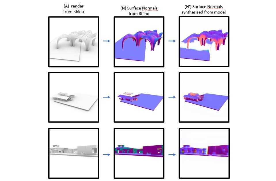
After a few hours of training, I try a few test images. Here are some cherry-picked examples that make it look like it’s working. The results are better when the input image resembles the Rhino rendered display mode used in training. While the model doesn’t have a strict comprehension of orientation, it’s generally grasped the concept that the main surface orientation is a light purple, and the perpendicular surfaces are pink and violet. It has a concept of white space being the unlabeled background.

This is an early proof of concept, with only 500 non-diverse training images, and a short training time, so I expect results to improve with subsequent trainings. I’m repeating this process with depth maps, line maps, and object segmentation. This should result in a set of Pix2PixHD models that can take any image and produce an imperfect set of custom drawing analyses. The goal is to use those analyses, and reverse the process to synthesize more realistic architectural drawings.
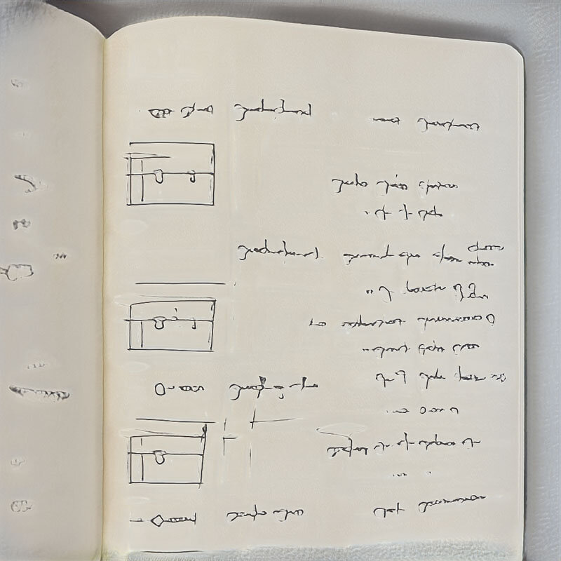
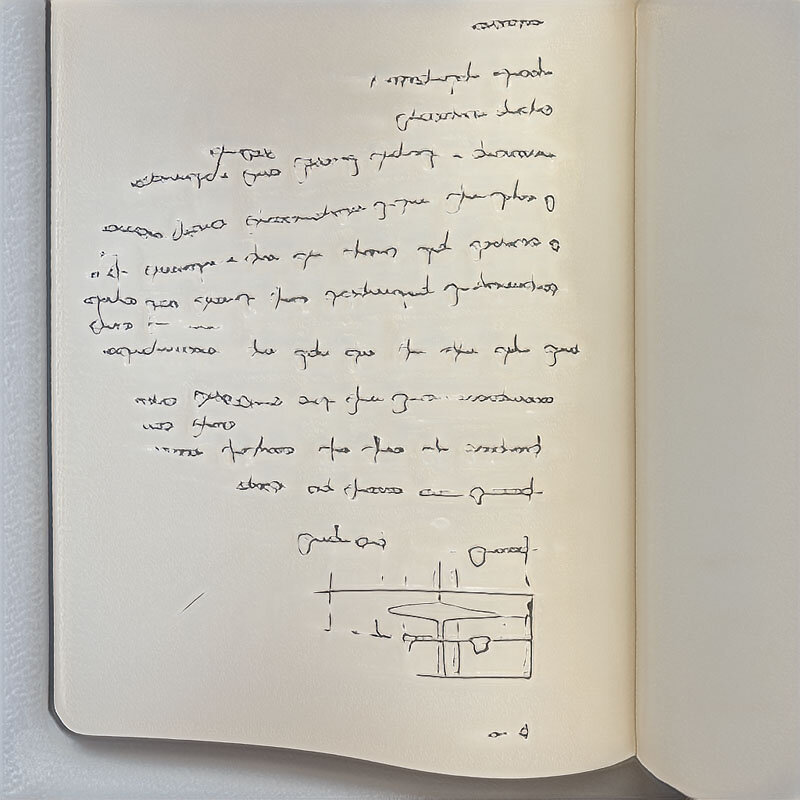
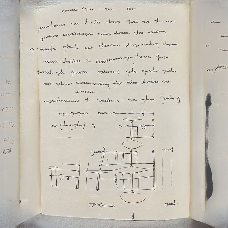
StyleGAN "Notebook"
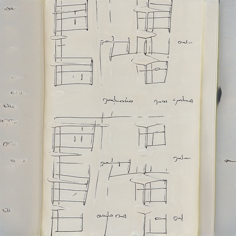
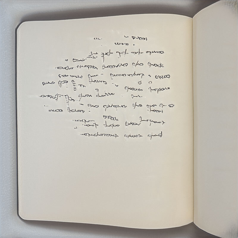
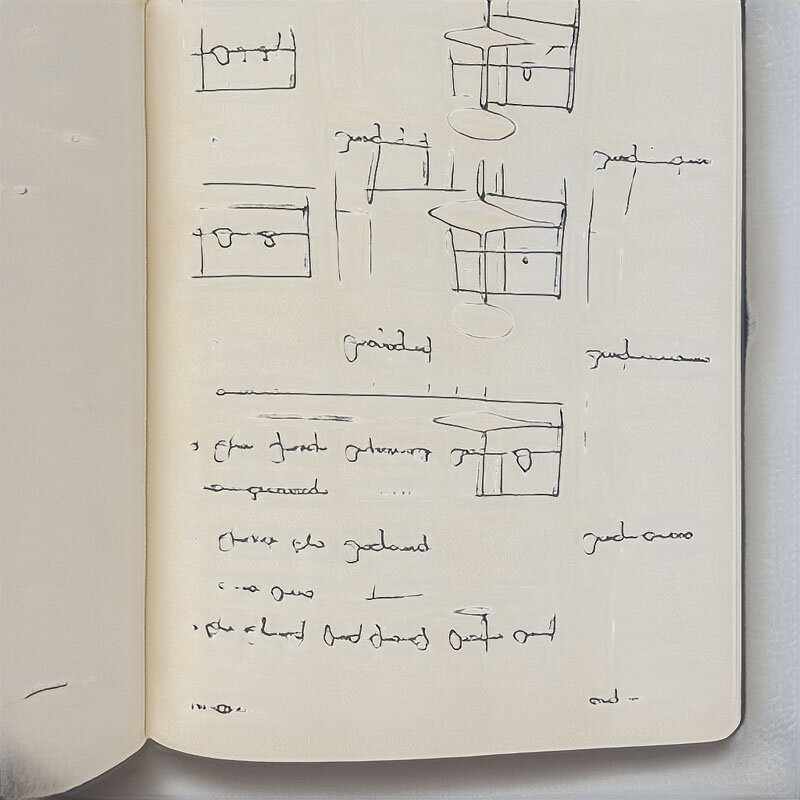
Results of a StyleGan2-ADA model, trained on 121 pages of one of my notebooks of architectural work from March 2020 to March 2021. The model picks up well on the character of my handwriting, and the overall composition of the page. I’m also impressed with how it renders the edges of the notebook. The drawings are a bit repetitive and lack imagination, but I’ll blame that on StyleGAN.


Play Pavilion at Margaret Hance Park
Earlier this month, a new playground opened at Margaret Hance Park in Phoenix, Arizona. This is the first phase of a larger revitalization of the park, and includes a small pavilion that I worked on with Lake Flato and Hargreaves Jones. This is a quick animation of the parametric design process.
The pavilion is a rusted steel structure that provides dappled shade to the sand pit below. It has a curved perimeter similar to the play area that it shades, and is just high enough that no one is tempted to climb on it. This gives us the overall area of the roof surface.
The pavilion surface is shaped as a section of a torus, so there’s some structural integrity in the curve of the surface, and the structure is curved along the same radius in two directions. This makes the beams easier to fabricate because the curve is identical at any point of the structure. The downside of this curved perimeter is that the perimeter beam becomes difficult to fabricate with double curvature. The perimeter beam was built in several sections and welded together.
Each steel plate is water-jet cut, placed, and welded on top of the structure. The circular perforations on the plates are arranged in the shape of several sunbursts, which provide dappled light to the sand pit.
This was a project that was very well-suited to be designed as a parametric model in Rhino and Grasshopper. The shape of the perimeter, placement of columns, size and spacing of beams, size and pattern of perforations, and many other variables were refined and reiterated countless times during the design process. Having the model set up as a system, and not as bespoke geometry made so much refinement possible.
This is the first of a few pavilions to be built in the park, and will hopefully see some use after Covid clears up and the sand pit is opened.

Photo by Jef Snyder
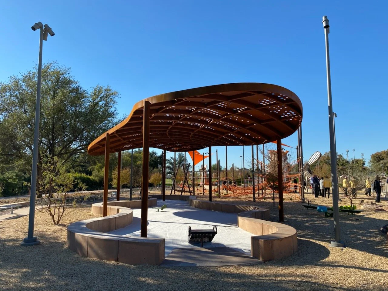
Photo by Jef Snyder
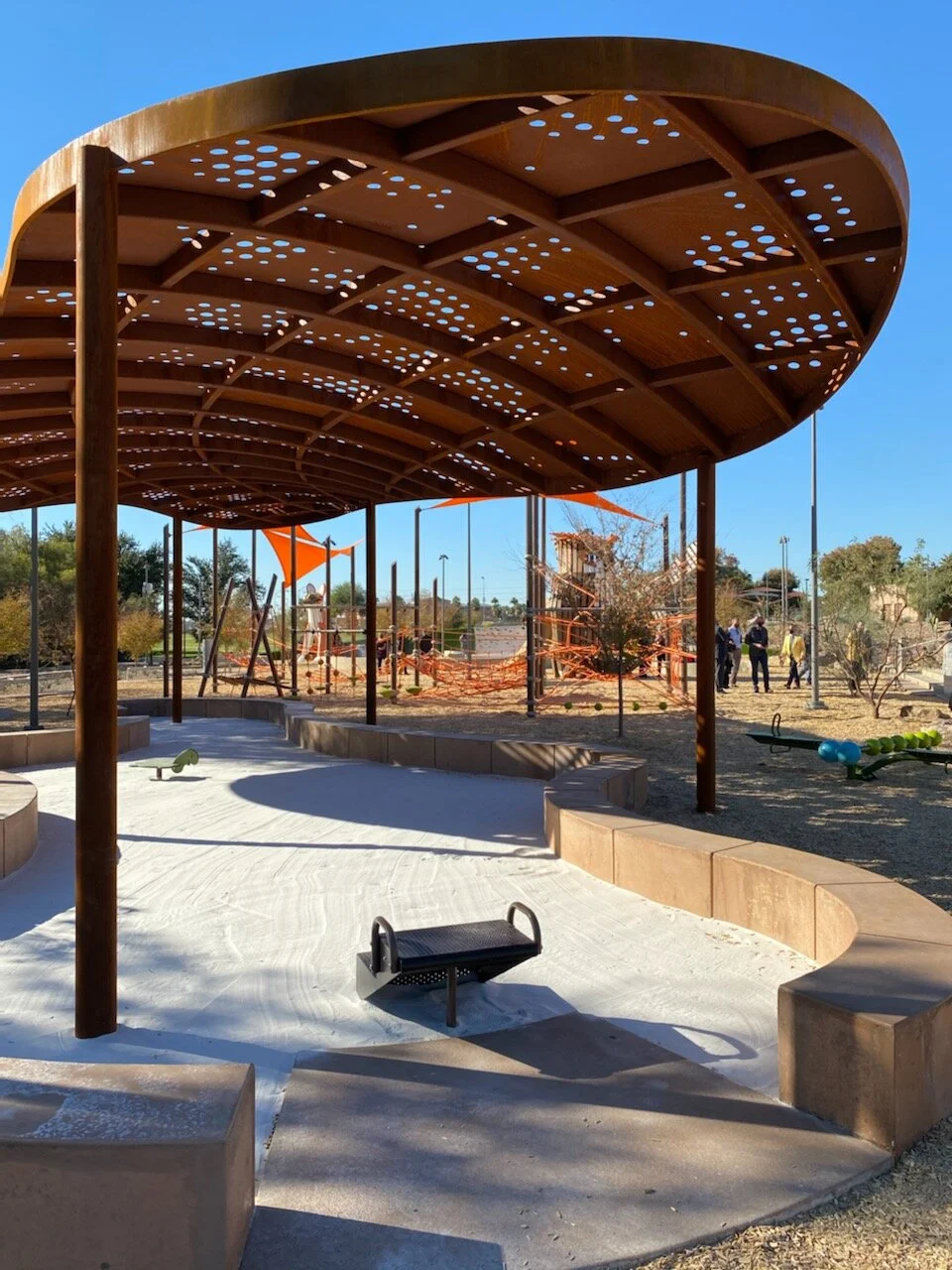
Photo by Jef Snyder
Moving Average - Grasshopper Component
This is a Grasshopper component that computes the moving average of a list of numbers. Input the list(s) and set the period (n). For the first few resulting values, this outputs the average of all the values so far, before a full period is reached.
Download here:
Read More5 Years of Shirts
For the last 5 years, I’ve recorded the color of the shirt I wear each day.
Read MorePseudo Non-Linear Regression in Grasshopper
I frequently need to use non-linear regression in Grasshopper, usually for interpolating data points on a 2D map. I frequently use the Non-Linear Regression component in Proving Ground’s LunchBoxML toolkit, but there are several occasions in which it’s challenging to set the right parameters to get the fit that I had in mind. This happens when the first two variables are so small or large (like with latitude and longitude) that the default sigma and complexity values in the LunchBoxML component are too far out of range to work. This script gives each test point a value based on the average of its closest points, then smooths out the data based on a confidence score.
Read MoreCity Roses - Graphic Tool for Visualizing Emotions
At the end of each day for the last few years, I’ve recorded data on 58 unique feelings, or affective states. I record everything I experienced on a scale of 0 to 10. Paired with data on where I was on each day, I can see a typical emotional profile of my experiences in each place.
Read More
Data-Driven Classification of Feelings
This is a method of classifying feelings based on 5 years of my self-reported data. At the end of each day, I record aspects of productivity such as sleep, diet, exercise, socializing, music, work, and learning, as well as 58 unique feelings, or affective states. These feelings are recorded on a scale of 0 to 10. This is an attempt at a data-driven classification of feelings, rather than thinking of all feelings as being either notionally positive or negative.
Does feeling (x) make me feel good or bad? Does feeling (x) make me more or less productive? Is feeling (x) more strongly associated with one behavior or another? This is a visualization of where each of those 58 feelings fall on a variety of spectra.
Each graph is a scatter plot that shows how strongly each of the 58 feelings are correlated with two other variables.
Read More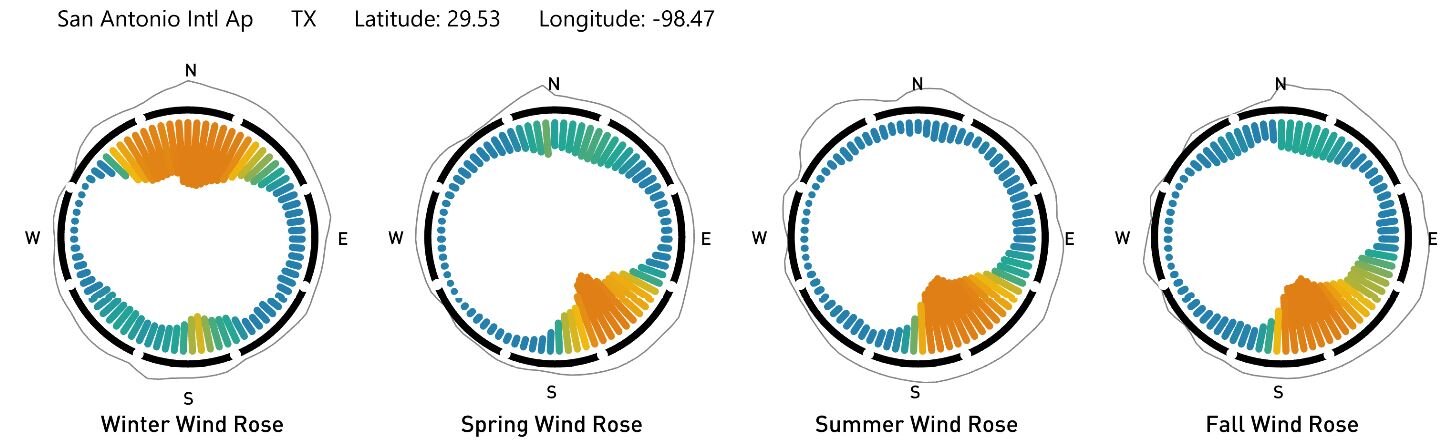
Automated Climate Graphics with Grasshopper
The automation of climate graphics is a great use case of parametric design. These graphs are the product of a collection of Grasshopper scripts that interpret a TMY3 weather file to produce a standard set of graphics.
Climate graphs, including wind roses, rainfall, humidity, heating/cooling degree days, temperature, cloud cover, and a psychometric chart.
Hourly thermal comfort graphs, which indicate the average temperature for every hour of the year, and whether or not each hour is above or below a given thermal comfort range.
Sun path and wind diagram, which indicates the position of the sun in the sky on key dates of the year, sunrise and sunset times, and the direction of the prevailing winds for each season.
Optimization Algorithms (Opossum) for Daylight Modeling
There are many design problems in architecture that lend themselves to parametric modeling. If a design can be defined by a few parameters (such as the height and depth of a light shelf), and evaluated with a few performance criteria (such as the useful daylight index of the room), then the design may be a good candidate for a parametric model. When these parameters are changed, the model instantly updates. A benefit of this setup is that a designer can use an optimization algorithm to discover the best possible combination of parameters to achieve a performance goal.
In this case, the parameters are the height and depth of both an interior light shelf and an external shade for a few different classrooms in a school in Houston. The performance criteria is an average of continuous daylight autonomy (cDA: the percentage of time the room is above 300 lux) and useful daylight index (UDI: the percentage of time the room is between 200 and 2,000 lux). This is a good balance of getting enough light to work with, while mitigating glare.
There are several types of optimization algorithms, such as genetic algorithms, simulated annealing, CMA-ES, and RBFOpt. Different types of algorithms have their own benefits. In this process, we are using the RBFOpt algorithm, because it is best at arriving at a good result with as few iterations as possible. This is important because each iteration of a daylight model may take several minutes. To find a reasonable solution quickly, we only have time to run about 20 or 30 iterations for each problem. I’m using DIVA for daylight modeling and Opossum 2.0; a Grasshopper component that runs RBFOpt and CMA-ES optimization algorithms.
Read MoreMobile Meshes - Drawing with Photogrammetry
This is a series of drawings that were made with COLMAP photogrammetry software and a grasshopper script. First, I take a video of a space as I walk through it. The video is usually 1 or 2 minutes long.
I take the video into Photoshop, and convert it into several still images using the Export > Render Video > Photoshop Image sequence tool.
I use COLMAP, a Structure from Motion pipeline to build a point cloud of the space from the image sequence.
I use a grasshopper script to export the point cloud from COLMAP file formats into Rhino.
Another script is used to connect the points in the point cloud depending on their proximity to each other. I export images of these meshes with varying density back into Photoshop and blend them.
Sometimes I use the real color of the scene, or exaggerate certain color families.
Biometric Mapping III
Biometric Mapping is a workflow that creates heat maps of the unseen qualities of spaces. For example: air quality data such as CO2, temperature, and humidity, or biometric data such as an occupant's heart rate, blood oxygen level, and neural activity.
Read More
Constructed Language in Grasshopper
This is an experiment in generating graphics that look like artificial written languages.
A typical way of constructing a written language is to start with a one-to-one transposition of existing letters into invented letters. This bottom-up approach may or may not produce cohesive looking text down the line when the characters are joined. Instead of starting with an alphabet, this alternate approach begins with a few rules for the composition of the characters, and then introduces random variations of those elements until the text as a whole looks convincing. From here, natural occurring and compelling fragments can be assigned to actual letters, and the alphabet can be post-rationalized.
Read More